Neural Turing Machine
Neural Turing Machine (NTM) is one of the first practices for utilizing an external memory to improve neural network performance; It aims to learn how to use a memory bank and act like a computer program to achieve a more generalized solution with fewer samples. This post discusses how NTM interacts and utilizes memory and tricks for a robust implementation.
Can Neural Network Learn Program?
Have you ever thought having a pen and piece of paper can help you in solving a problem?
Have you ever write a program that can do better only by having more amount of memory?
Having more paper doesn’t make you smarter (does it?), you are the one who knows how utilize the pen and paper to split a complex problem to simple steps.
The same story goes for Neural Networks. We leave them to solve our problems without any pen or paper, and it leads to an unnatural way of learning that usually is not Robust, Scalable, and needs a Massive amount of samples.
Alex Graves(DeepMind) claims this in his paper on NTM:
We extend the capabilities of neural networks by coupling them to external memory resources, which they can interact with by attentional processes.
But there’s no official implementation of his work, so in this post, we discuss how NTM works and in the next post I present a robust implementation of NTM that trained on different tasks and achieved performance near what was reported in the original paper.
- Motivation
- Inspiration
- Intuition
- Mathematics
- Implementation
- Experiment & Result
- Conclusion
- Future Works
- Appendix: Various Implementation of NTM
- References
Motivation
When we face complex problems: On the one hand, we can train a large-scale deep learning model, which is not so natural. Therefore, we need a massive amount of data to train specific tasks with no ability to generalize or deal with noises. On the other hand, we have good old symbolic AI, which cannot keep up in accuracy and speed with Neural Network, but understandable and robust.
From the early days of Neural Network (when they call it connectivisim approach or distributed data processing), symbolic AI scientist raises to critics:
- Incapable of handling variable-sized input
- Incapable of “variable-binding” (e.g. Mary Spokes to John; we bind Mary to subject role.)
After some years, Recurrent architecture appears and solved the first critic. Still, Neural Network cannot bind variables, one of the critical requirements of any computer algorithm. The NTM aims to solve this second critic.
Inspiration
In the NTM paper, the first source of inspiration comes from Neuroscience and Psychology; It claims that even humans have a Working Memory to handle variable binding and known as Rapidly Created Variables.
The second inspiration comes from Turing Machine (Von Neumann architecture). It shows that even a simple Finite-State Machine (Controller) with infinity tape (Large enough memory) can simulate any algorithm.
Neural network architecture can also solve complex problems using simple architecture and memory instead of a large complex architecture.
Intuition
The below figure is how a simple Von Neumann Architecture looks like:
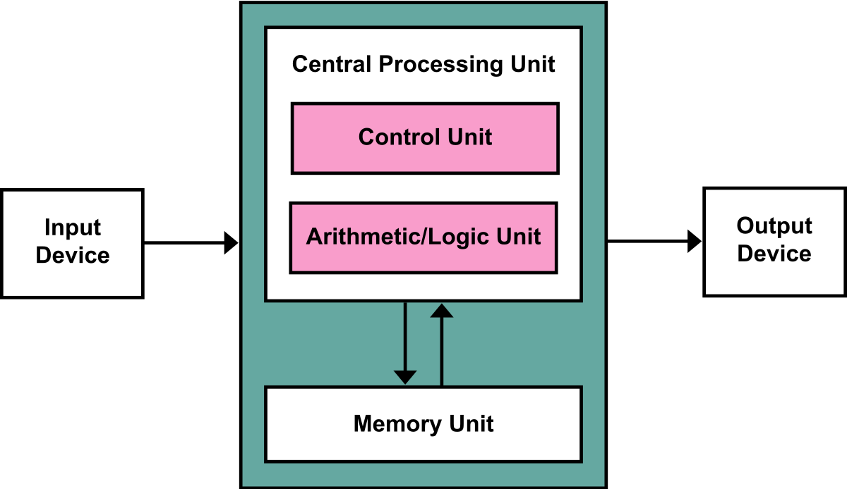
Figure 1. CPU interacts with memory to process inputs and generate outputs. (Image source: Wikipedia)
By this idea, we can assume the NTM as follow:
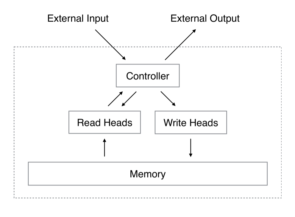
Figure 2. NN controller interacts with memory with the help of reading/Write heads like Turing Machine. (Image source: Original Paper)
Mathematics
First, we discuss how we can read, write, and address memory in a differentiable manner. Then, we discuss how a Neural Network can generate addresses and information that suit this memory.
Memory
The Memory is a matrix with the size of \({m \times n}\). We show it in time \(t\) as \(M_t\) For reading in a differentiable manner from memory. We define the address as a distribution of rows of the matrix, and output will be the expected value of address over the memory’s content. the \(w_t(i)\) is addressed in the form of:
\[\sum_i{w_t(i)} = 1\\ 0 \le w_t(i) < 1, i \in (0, ..., m-1)\]and we have \(r_t\) the read vector of memory as:
\[r_t \leftarrow \sum_i{w_t(i)M_t(i)}\]similar to read, we can define the write, with two additional vectors for add \(a_t\) and erase \(e_t\).
\[\tilde{M}_t \leftarrow M_{t-1}(i)[1 - w_t(i)e_t],\\ M_t(i) \leftarrow \tilde{M}_t + w_t(i)a_t.\]It can as read and write heads use simple attention method to interact with memory.
Heads
Now we look into a more important part: Addressing!
-
Focusing by content: The first step to address a memory location is to use similarity between memory values and controller output; this approach seems like searching inside memory to find a close match for a query. At the time \(t\) each head produce a key-strength \(\beta\) and a key-vector \(k_t\) of length \(m\). The address (distribution) can be generated as follows:
\[w^c_t(i) \leftarrow \frac{\exp{(\beta_tK[k_t, M_t(i)]}}{\sum_j \exp{(\beta_tK[k_t, M_t(j)])}} \leftarrow Softmax(\beta_tK[k_t, M_t(i)])\\ K[u,v] = \frac{u.v}{||u|| . ||v||} \leftarrow \textbf{ Cosine Similarity }\]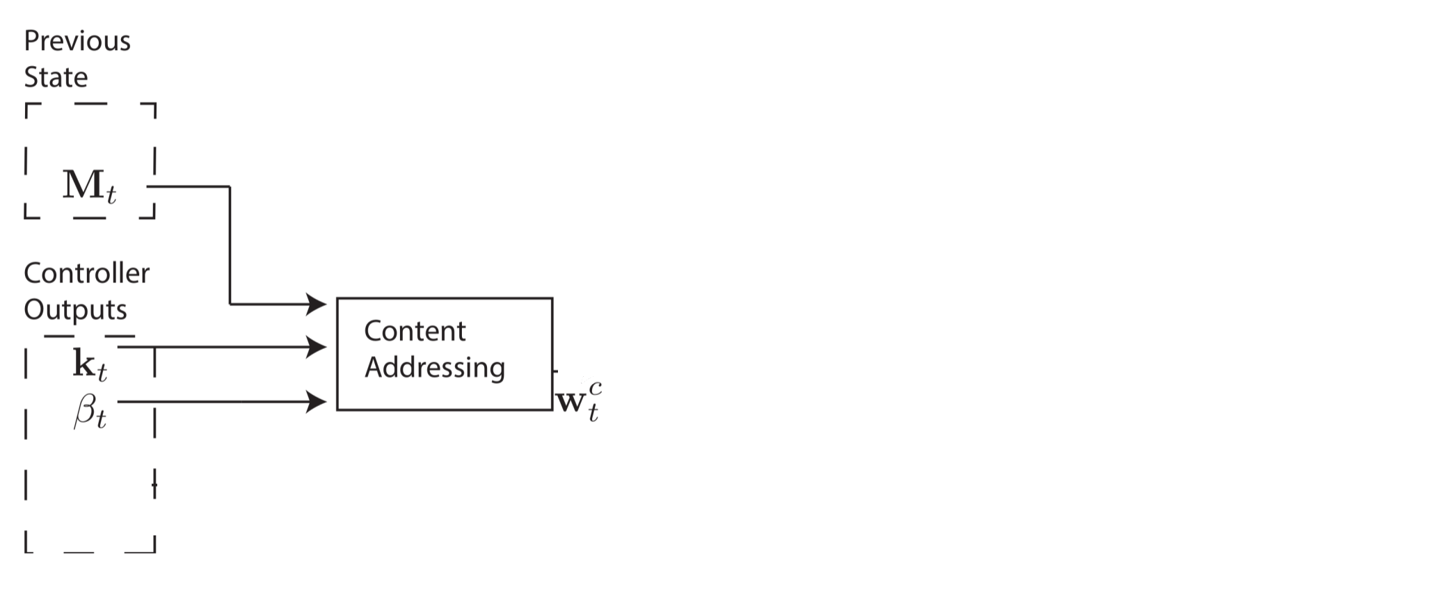
Figure 3. Addressing By Content Similarity. (Image source: Original Paper)
-
Interpolation In the second step, we controller the ability to Interpolate the address between the last address and new address; this Interpolation decide by one gate value \(g_t\) an it goes as follows:
\[w^g_t \leftarrow g_tw^c_t + (1 - g_t)w_{t-1}.\]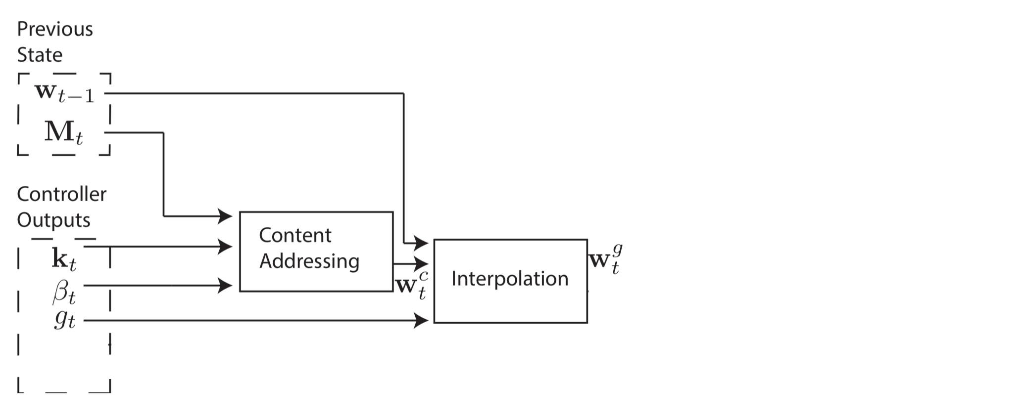
Figure 4. Interpolation of Address. (Image source: Original Paper)
-
Convolutional Shift This step creates the ability to shift the Interpolated address, which helps iteration over memory cells or get a value before/after the query. each head decide the shift amount by generating a distribution over allowable shift values (i.e. [-2, -1, 0, 1, 2]) as \(s_t\).
\[w^s_t \leftarrow \sum^{n-1}_{j=0}w^g_t(j)s_t(i - j)\]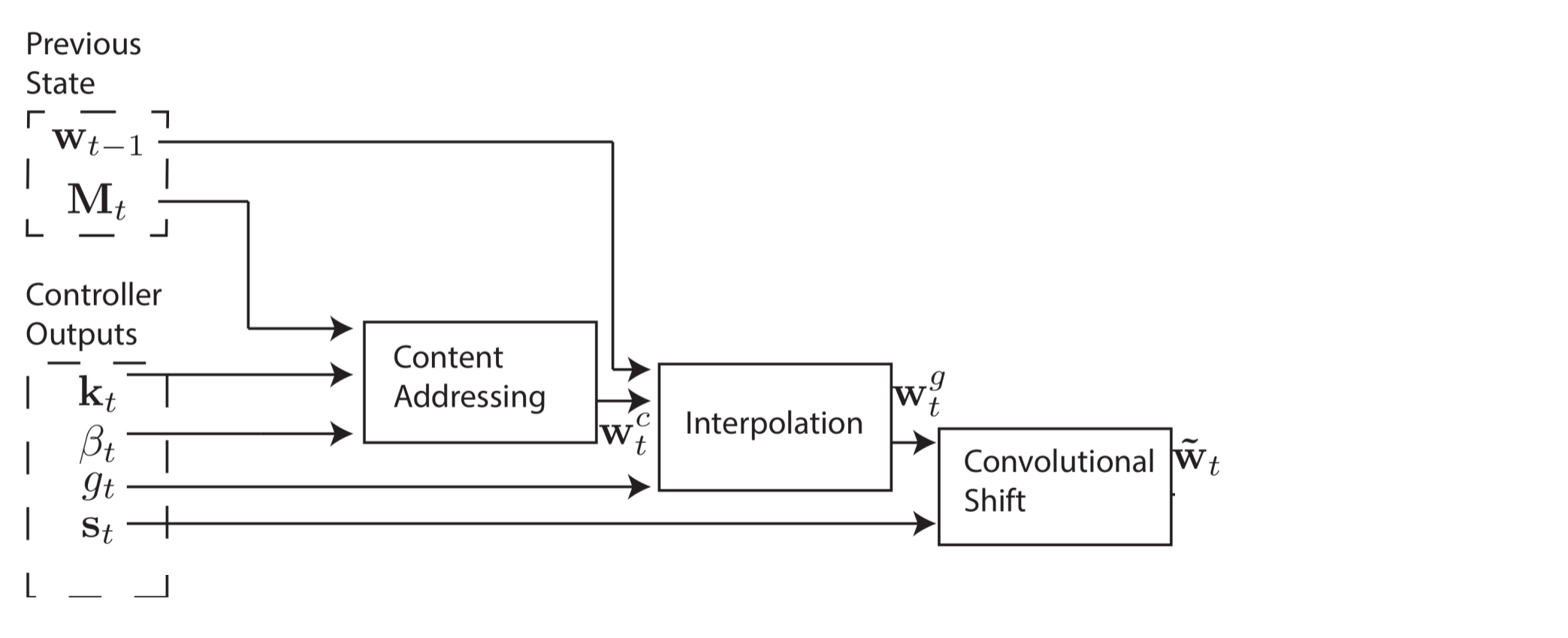
Figure 5. Shifting the Address by Convolution. (Image source: Original Paper)
-
Sharpening We need a differentiable way to apply the shift, so we used the Convolutional Shift in the last step, but the Convolutional shift also makes the output vector blurry, so reduce this blurriness, there’s a sharpening step after shift, and power of sharpening is decided by \(\gamma_t\).
\[w_t \leftarrow \frac{w^s_t(i)^{\gamma_t}}{\sum_j{w^s_t(j)^{\gamma_t}}}\]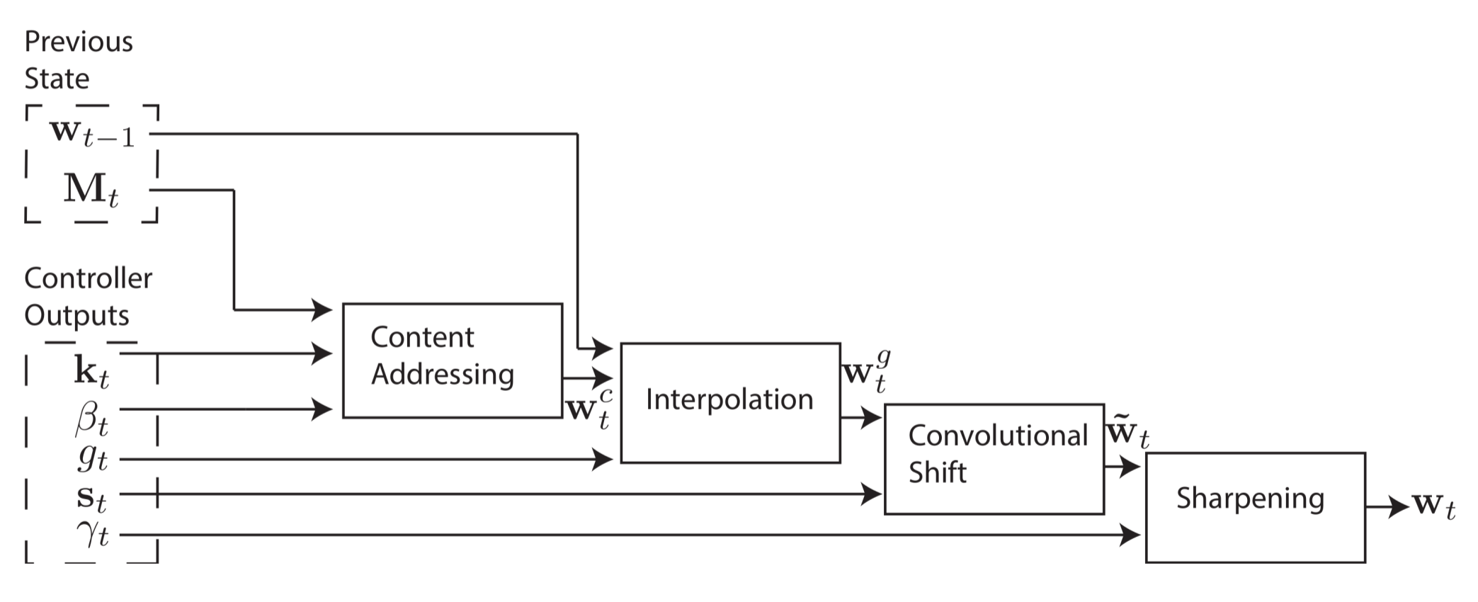
Figure 6. Sharpening of Shifted Address. (Image source: Original Paper)
And that’s it! the distribution vector \(w_t\) is generated for each head based on the last state of memory and controller output, the system is entirely differentiable and thus end-to-end trainable.
controller
The controller can be any NN; the paper test how Feed-Forward or RNN perform on different tasks. Besides the final results, the paper makes the following statements:
- The LSTM version of RNN has an internal memory that acts like registers of the processor.
- LSTM mix information across multiple time-steps so the task can be done with fewer heads.
- Feed-Forward has better transparency, which only relays on external memory.
Implementation
They say you didn’t understand it unless you can explain it well, I believe in CS: you didn’t understand it unless you implement it well, As there was no official implementation for this paper, I was eager to do it myself and see what can go wrong, and as I expected anything that can go wrong, I learned few tricks to make it robust and fast. I explain the code and implementation with PyTorch in another post, but we focus on concepts for now.
-
Base Architecture Here’s what I understood after reading the paper, I decide on those activation functions respected to bounds and behavior of variables. Seems good, doesn’t work!
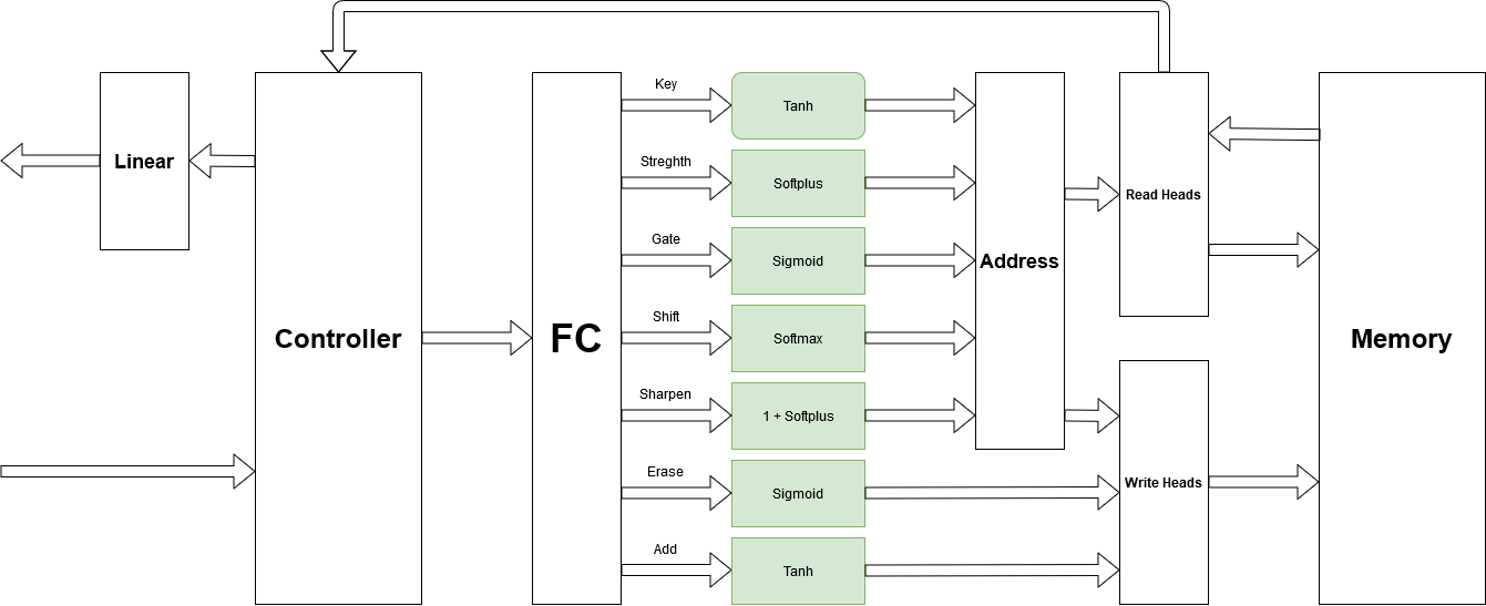
Figure 7. NTM Architecture Level1.
-
Moore to Mealy. The first trick is to improve the speed of training, and also robustness was changing from Moore to mealy, which means that the state of the controller can decide on output and current values of read heads should be involved.
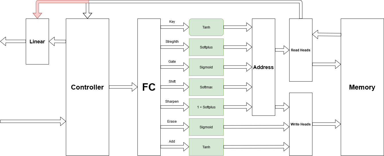
Figure 8. Adding Path between read head and ootput
-
Split the FC!. Yes! It helps a lot and has brings performance improvement.
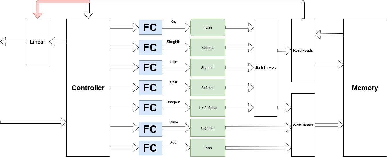
Figure 9. Split Fully Connected Layer
-
Clip output and gradient. This is very important in the robustness of training; otherwise, you may face g radiant exploit. I tried to clip it in the range of \([-10, 10]\) and works fine.
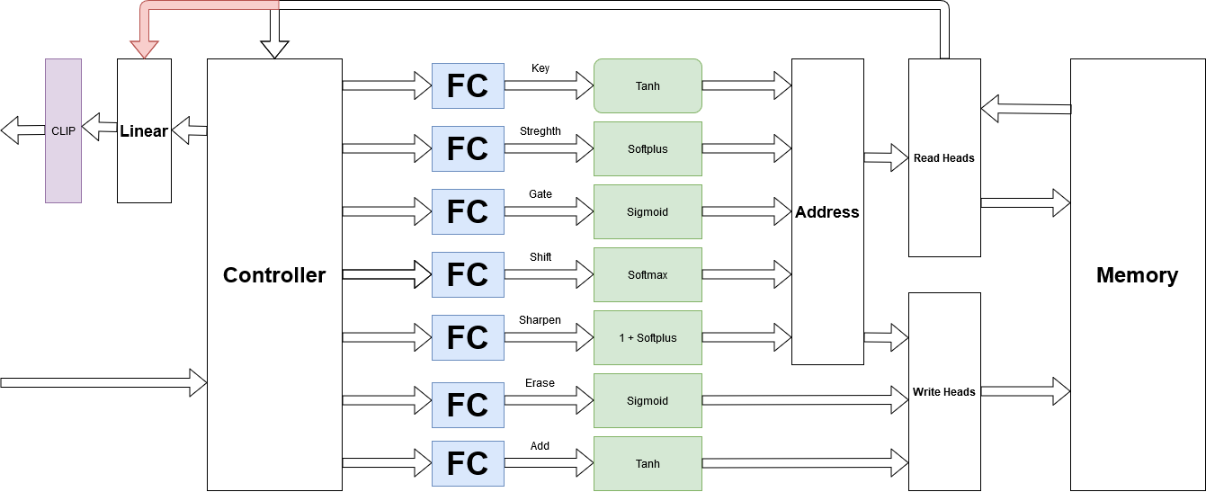
Figure 10. Clip gradient and outputs
-
Initialization Matters. The initial values of memory and heads matter a lot in training; Collier et al. 2018 compared the performance of different Initialization; here’s what I understand: you should either go with constant Initialization of memory and trainable Initialization for heads or initialize everything uniformly random. (I did the second one, but first is recommended).
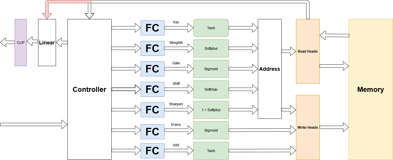
Figure 11. Distribution of initialization of memory and heads matters
Experiment & Result
The paper suggests five tasks, which I implement and test four of them.
- Copy Task
- Repeated Copy Tasks
- Associative Recall
- Priority Sort
Before jumping to plots and graphs, I want to recall what we expected to see in these results:
- Can NTM learn more Natural? (e.g. fewer samples)
- Can NTM Generalize beyond the training range?
- How NTM utilize memory at all?
Can NTM learn more Natural?
Firstly, there is the comparison of NTM and LSTM in different tasks to see how faster NTM learns.
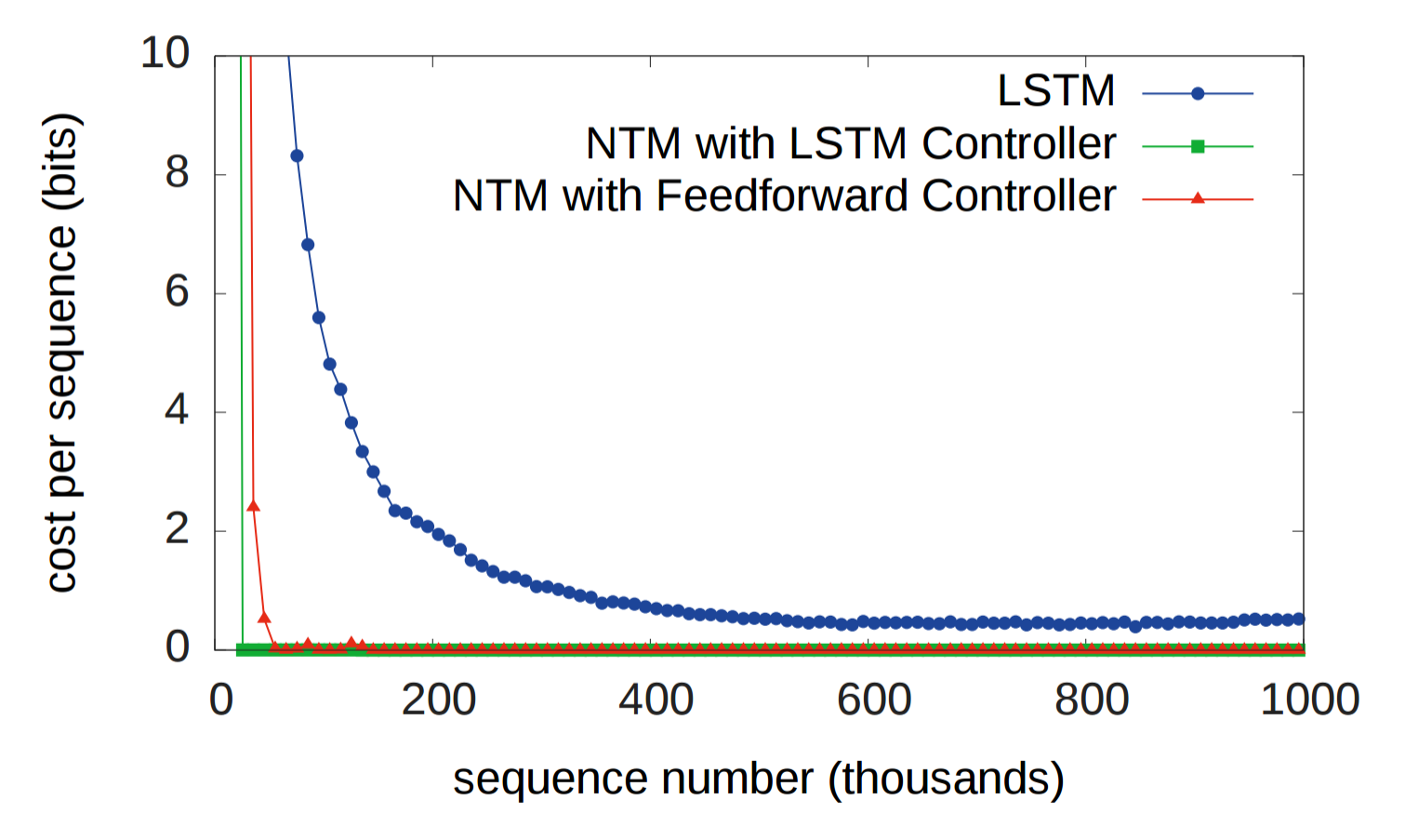
Figure 12. NTM and LSTM learning curve for copy task
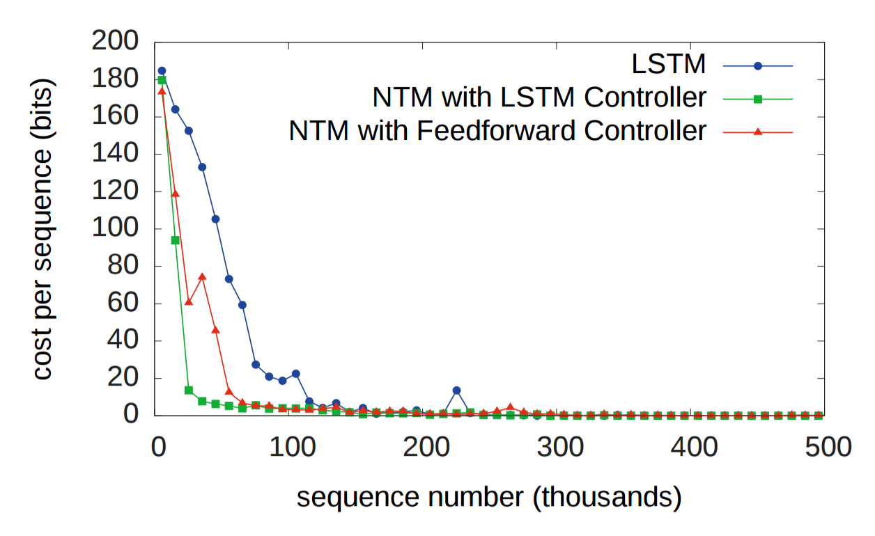
Figure 13. NTM and LSTM learning curve for repeat copy task
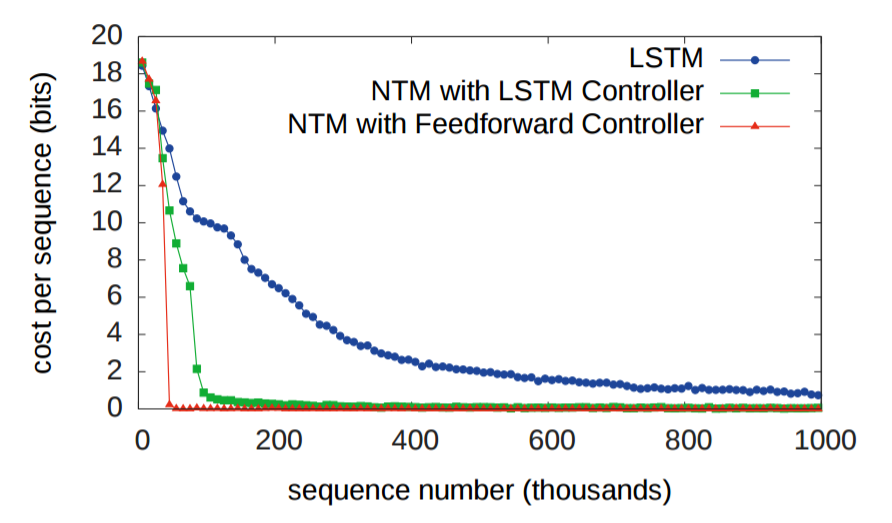
Figure 14.NTM and LSTM learning curve for associative recall task
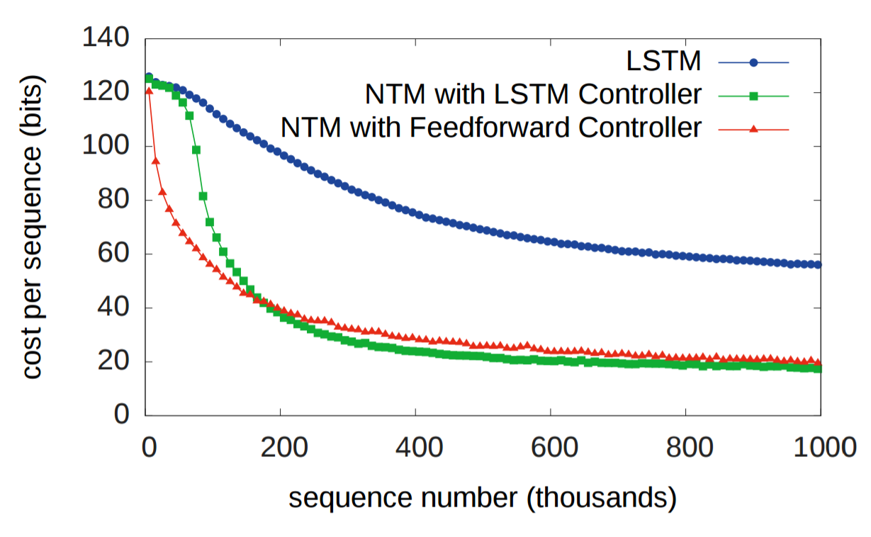
Figure 15.NTM and LSTM learning curve for priority sort task
Can NTM Generalize beyond the training range?
Second, how good NTM can generalize the out of training range:
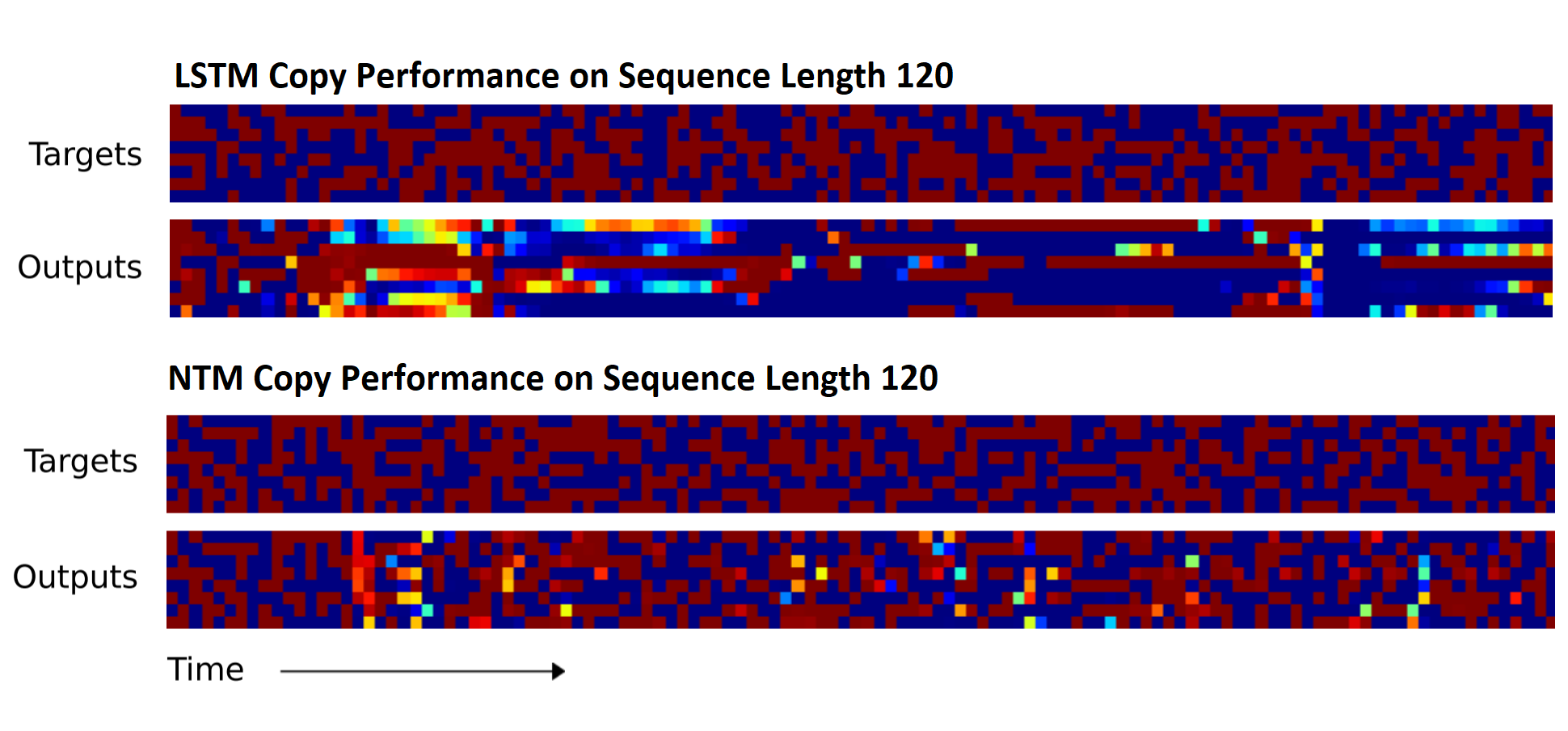
Figure 16. NTM and LSTM Generalization performance on Copy Task (Train for 10, Test for 120)
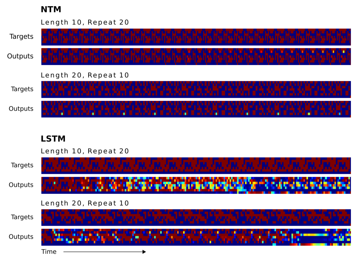
Figure 17. NTM and LSTM Generalization performance on Repeat Copy Task (Train for 3, Test for 20)
How NTM utilize memory at all?
Third, the way NTM utilized the memory is the same as a programmer wants to use the memory for the copy task. This similarity may recall from the fact that NTM is learning a program instead of a function estimator.
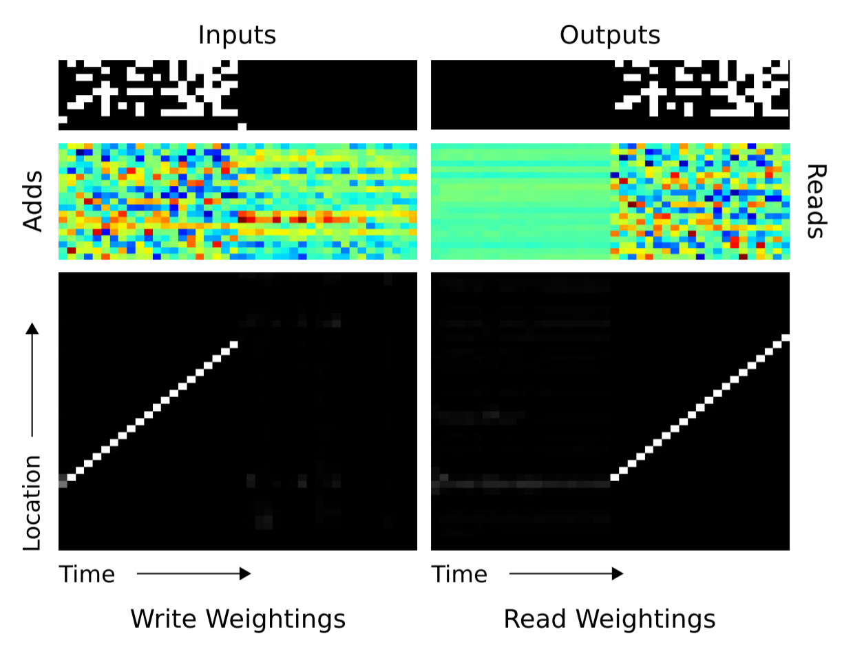
Figure 18. Memory Read/Write heat map trough time. (Image source: Original Paper)
Conclusion
In conclusion, the idea from neuroscience and computer architecture suggest using external memory as a possible solution to a scathing criticism of connectionism (variable-binding). NTM needs blurry reads and writes to learn how to use memory and outperform and learn more generalizable algorithms than LSTM. NTM memory access is natural (Is it learning algorithm?).
Future Works
Any Drawbacks of NTM?
- NTM Lacks the support for pointer and data structures
- No link between data or ability to backtrack
- There’s no way to unallocate memory
Mostly solved in by the same authors in DNC architecture.
My Open Questions?
- What is the actual role of memory in deep learning?
- How can memory be traded with learnable parameters?
- What is the best way to utilize memory?
- How is the data encoded, stored, and extracted in the memory?
- Can we learn the memory size and structures too?
Appendix: Various Implementation of NTM
-
MarkPKCollier/NeuralTuringMachine: a stable Tensorflow implementation of a NTM.
-
loudinthecloud/pytorch-ntm: PyTorch implementation of Neural Turing Machines (NTM).
-
snowkylin/ntm: TensorFlow implementation of Neural Turing Machines (NTM), as well as its application on one-shot learning (MANN).
References
[1] Graves, Alex, Greg Wayne, and Ivo Danihelka. “Neural turing machines.” arXiv preprint arXiv:1410.5401 (2014).
[2] Collier, Mark, and Joeran Beel. “Implementing neural turing machines.” International Conference on Artificial Neural Networks. Springer, Cham, 2018.
[3] Graves, Alex, et al. “Hybrid computing using a neural network with dynamic external memory.” Nature 538.7626 (2016): 471-476.